1. Introduction: From Noise to Narratives
In its rawest form, data is often nothing more than a chaotic collection of disconnected facts—numbers in a spreadsheet or labels in a database. Without structure, these points are silent. Descriptive statistics serves as the “grammar and syntax” of this world, providing the tools necessary to translate chaos into structured knowledge. It is, in essence, the art of storytelling with numbers.
To understand your role as a data analyst, consider the Foundational Analogy of a novel:
- Descriptive Statistics (The “Book Report”): This is akin to writing a factual, detailed report after reading a book from cover to cover. You have all the information in front of you, allowing you to state with 100% certainty the average chapter length or the most frequent word. You are describing a known entity with zero ambiguity.
- Inferential Statistics (The “Literary Prophet”): This is like reading only the first chapter and trying to predict the entire plot. You use a small sample to make an “educated guess” about the whole story. This process inherently involves probability and uncertainty.
The “So What”: Why must mastery of the “critic” (description) precede the “prophet” (inference)? Because inference is an educated guess built upon the foundation of your sample. If you cannot describe that sample perfectly, your predictions about the larger population are built on sand. Before you can predict the future of a story, you must be able to accurately summarize the chapters you have already read.
Throughout this guide, we will step into our Laboratory: a case study featuring a dataset of 2,392 high school students. These students are the “characters” in our story. By looking at their demographics (Ethnicity), habits (Absences), and outcomes (GPA), we will see how data classification dictates the way we tell their tales.
Before we can begin the storytelling process, we must first learn to classify our characters by identifying the two primary families of data.
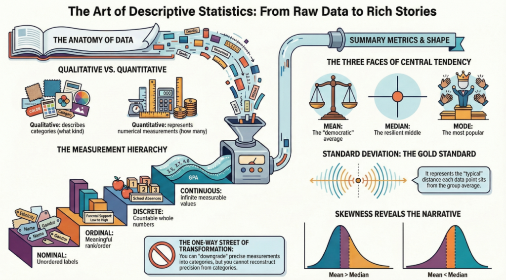
2. The Great Divide: Qualitative vs. Quantitative Families
All data belongs to one of two broad families. Your first task is to identify the core question the data answers: “What kind?” or “How much?”
The Two Families of Data
| Family Name | Core Definition | Case Study Example |
| Qualitative (Categorical) | Describes qualities, characteristics, or labels. Answers “What kind?“ | Ethnicity (e.g., Caucasian, Asian, African American) |
| Quantitative (Numerical) | Represents a measurement or a count. Answers “How much?” or “How many?“ | GPA (e.g., 3.5, 3.8) |
A common trap I see students fall into is assuming that any variable containing a number is quantitative. To avoid this, ask yourself: Can I perform meaningful math on this number?
For instance, a student’s Postcode or a Coded Gender (0 for Male, 1 for Female) uses numbers, but calculating the “average” postcode is nonsensical. These numbers are merely labels. If the math doesn’t make sense, the data is Qualitative.
Once you have identified the family, we must look closer at the specific “species” within that group to understand their unique properties.
3. The Qualitative Realm: Names and Ranks
Qualitative data is divided into two species based on whether the categories have a natural order: Nominal and Ordinal.
Nominal Data
The term Nominal comes from the Latin root nomen, meaning “name.” These variables are essentially just named labels.
Nominal data consists of categories with no intrinsic order or ranking. Think of school subjects like “Mathematics,” “History,” and “Art.” They are distinct, but one does not “rank” higher than the other in a natural hierarchy.
Ordinal Data
Ordinal data involves categories where the order matters, but the “distance” between the ranks is unknown or inconsistent.
The Limitation of Gaps: Think of a satisfaction survey (Dissatisfied, Neutral, Satisfied). While we know “Satisfied” is better than “Neutral,” we cannot mathematically prove the “gap” in satisfaction is equal. In our case study, consider ParentalEducation. The effort required to move from “None” to “High School” is not necessarily the same as the move from “High School” to “Bachelor’s Degree.” The order is clear, but the intervals are not.
Case Study Spotlight
- Ethnicity (Nominal): Coded as 0, 1, or 2, these are arbitrary labels. Being coded as “2” does not imply “more” ethnicity than a “0.”
- ParentalSupport (Ordinal): Coded from 0 (None) to 4 (Very High). There is a meaningful order—Very High is clearly more than Moderate—but we cannot quantify the exact “amount” of support that separates each level.
While qualitative data relies on labels, quantitative data provides the precision of numerical measurements.
4. The Quantitative Realm: Counting vs. Measuring
Quantitative data is split into Discrete and Continuous species, determined by whether the values are separate points or exist on a fluid scale.
Discrete vs. Continuous Data
| Characteristic | Discrete Data | Continuous Data |
| Core Definition | Countable items with specific, distinct values. | Values that can take any point within a range. |
| Key Property | Finite Gaps: You cannot have a value between the steps. | Fluid Scales: Infinite possible values, limited only by the precision of the instrument. |
| Analogy | Classroom Students: You can have 25 or 26 students, but never 25.5. | Measuring Height: A student might be 165 cm, or 165.112 cm, depending on the ruler used. |
| Case Study Example | Absences: A student missed 5 days or 6 days, not 5.27 days. | StudyTimeWeekly: A student could study 5 hours, 5.1 hours, or 5.15 hours. |
These four types are not just separate categories; they exist within a specific power structure that dictates your entire analytical strategy.
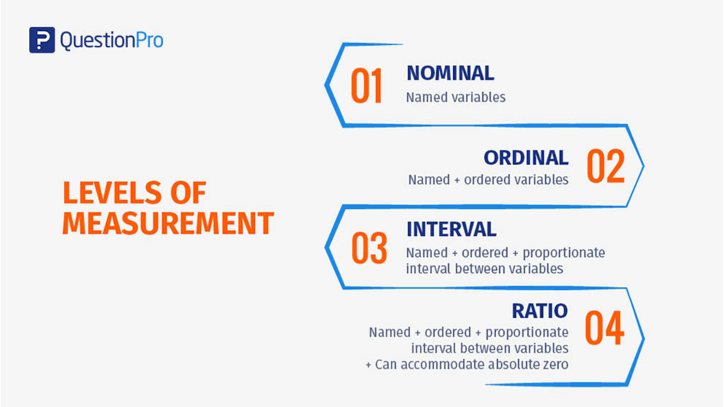
5. The Hierarchy of Data: The One-Way Street
Data types follow a clear measurement hierarchy: Nominal < Ordinal < Quantitative. Each step up the ladder adds a new property:
- Nominal: Provides a label.
- Ordinal: Adds Order.
- Quantitative: Adds Consistent, meaningful intervals.
The Strategic Lesson: Risk Management
Think of this hierarchy as a one-way street. You can always downgrade data, but you can never upgrade it. This is a vital lesson in research strategy.
In our case study, a precise GPA (Quantitative) can be grouped into Grade Classes like ‘A’ or ‘B’ (Ordinal). This “coarsening” of data is often done for simplicity. However, if you only collect the “Grade Class” to begin with, you can never go back and find the student’s exact GPA. The nuanced information is lost forever.
The Mentor’s Rule: Always collect data at the highest level of precision possible (Quantitative) to maintain maximum flexibility later.
To help you navigate these classifications in practice, use the following matrix as your primary reference tool.
6. The Data Specialist’s Quick-Reference Matrix
| Data Type | Core Definition | Case Study Example | Appropriate Descriptive Tools |
| Nominal | Unordered categories or labels. | Ethnicity | Mode, Frequency Tables, Percentages, Bar/Pie Charts |
| Ordinal | Ordered categories with undefined intervals. | ParentalSupport | Median, Mode, Percentiles, Quartiles, Bar Charts |
| Discrete | Countable, distinct numerical values. | Absences | Mean, Median, Mode, Standard Deviation, Variance, Histograms |
| Continuous | Measurable values on a fluid scale. | GPA | Mean, Median, Standard Deviation, Variance, Histograms, Box Plots |
7. Conclusion: Building a Solid Foundation
Mastering the anatomy of data is the first and most critical step in your journey. As a mentor, I cannot overstate this: misclassifying your data doesn’t just lead to a minor error—it risks making your entire subsequent analysis invalid.
By correctly identifying whether your data is Qualitative or Quantitative, and recognizing its place in the Hierarchy of Data, you empower yourself to choose the right tools for the job. You are no longer just looking at a spreadsheet of 2,392 students; you have cracked the code of their language. You are now the expert literary critic, ready to weave a factual, insightful, and powerful story from the characters within your data.